XYmath does curve fitting
XYmath will find the “best” curve fit using either minimum percent error or minimum total error. It can search through common equations, an exhaustive search through thousands of equations, splines, smoothed splines, or non-linear equations input by the user.
After fitting, XYmath will find roots, minima, maxima, derivatives or integrals of the curve. It will generate source code that documents and evaluates the fit in python, FORTRAN or EXCEL.
Configurable plots are created using matplotlib that are of publication quality.
Basic Usage
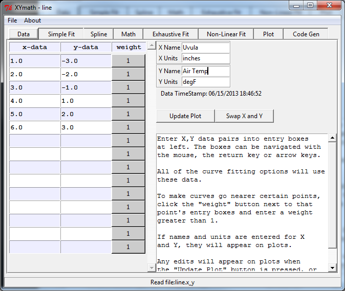
The interface consists of tabbed pages for each of the major functions. The data entry page below shows all of the tabs.
- Data - for entering X,Y data and data definitions
- Simple Fit - fits the data to common equations and ranks them
- Spline - fits the data to one of several splines
- Math - performs min/max, derivative, integration, root finding on curve fit
- Exhaustive Fit - searches hundreds or millions of equations for best fit
- Non-Linear Fit - fits data to a user-defined, non-linear equation
- Plot - provides plotting options
- Code Gen - generates python, FORTRAN or Excel code to document and implement curve fit
There is a “Show Help” button on most pages to provide guidance.
Installing XYmath
If a recent version of pythonxy is installed, then XYmath can be installed with no additional dependencies. XYmath makes use of a number of packages that come with pythonxy like numpy, scipy, matplotlib and numexpr. XYmath itself is a pure python package, all modules are written in python with no compiled extension modules of its own.
Pythonxy can be found at: https://code.google.com/p/pythonxy/
XYmath was developed with python 2.7 requires modules:
Simply download and execute the EXE installation file. For version X.X.X that would be the file XYmath-X.X.X.win32.exe
If you prefer to install from source code, download XYmath.X.X.X.zip, unzip and run “setup.py install”
Running XYmath
The setup script places the file “xymath.bat” into the main python directory such that typing “xymath” at the command prompt will launch XYmath (assuming that C:\python27 is in your PATH).
As an alternative, you can run the script “make_xymath_shortcut.py” located in “C:\Python27\Lib\site-packages\xymath” and a desktop shortcut will be created.
If there is an existing XYmath dataset file (e.g. mydata.x_y), the command “xymath mydata” will launch XYmath and open the dataset, or drag and drop mydata.x_y to the desktop icon created above.
Entering Data
The form for entering X,Y data is shown below. Enter X,Y data pairs into entry boxes. The boxes can be navigated with the mouse, the return key or arrow keys.
All of the curve fitting options will use these data.
To make curves go nearer certain points, click the “weight” button next to that point’s entry boxes and enter a weight greater than 1.
If names and units are entered for X and Y, they will appear on plots.
Any edits will appear on plots when the “Update Plot” button is pressed, or when another tabbed page is selected.
Simple Fit
The X,Y data can be fit to equations by minimizing either total error, or percent error. Selecting the “Total Error” or “Percent Error” radio button at upper left will determine which approach is used.
A limited set of common equations with 1 to 4 terms on the right hand side is fit to the data when the “Curve Fit” button is pressed.
If fewer than 4 terms are desired, the “Max Terms” can be reduced from 4 to the desired number.
All of the equations are listed in order from best to worst standard deviation or percent standard deviation as appropriate.
Note that for some equations, divide by zero is allowed if it results in (1/infinity) which is equal to 0.0
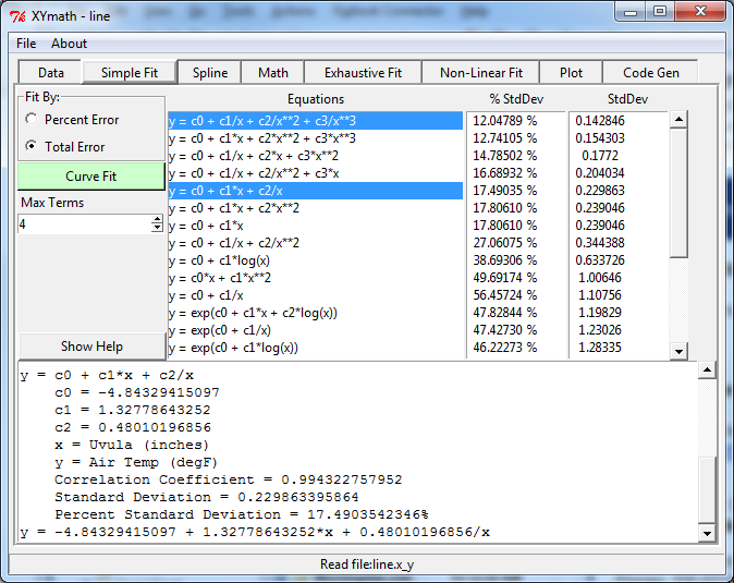
The equations in “Simple Fit” are:
y = c0 + c1*x + c2*x**2 + c3*x**3 <-- CUBIC POLYNOMIAL
y = c0 + c1/x + c2*x + c3*x**2
y = c0 + c1/x + c2/x**2 + c3*x
y = c0 + c1/x + c2/x**2 + c3/x**3
y = c0 + c1*x + c2*x**2   <-- QUADRATIC POLYNOMIAL
y = c0 + c1*x + c2/x
y = c0 + c1/x + c2/x**2
y = 1/(c0 + c1/x + c2*x)
y = exp(c0 + c1*x + c2*log(x))
y = c0 + c1*x          <-- STRAIGHT LINE
y = c0 + c1/x
y = c0*x + c1*x**2     <-- QUADRATIC THROUGH ORIGIN
y = c0 + c1*log(x)
y = 1/(c0 + c1*x)      <-- STRAIGHT LINE FOR 1/y
y = 1/(c0 + c1/x)
y = 1/(c0 + c1*log(x))
y = 1/(c0*x + c1/x)
y = exp(c0 + c1*log(x))  <-- LINEARIZED EXPONENTIAL y=A*x**n
y = exp(c0 + c1/x)
y = exp(c0 + c1*x)
y = c0*x           <-- STRAIGHT LINE THROUGH ORIGIN
y = c0/x
y = c0   <-- MEAN OR WEIGHTED MEAN
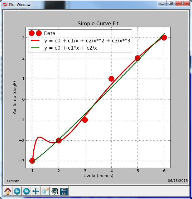
Notice on the plot below that two different equations were selected and plotted.
Splines
Spline curves can go through all data points or be smoothed to give an approximation of the data. To create spline curve fit:
- Select the desired spline, or splines (order 1 to 5, Linear to Quintic)
- Select any desired “smoothing”
If smoothing is equal to zero, the spline will go through all data points.
With smoothing added, the curve will go near the data points, but not necessarily through them. Click the Smoothing spin box to change the amount of smoothing.
Standard deviation and percent standard deviation will be calculated for smoothed splines along with their correlation coefficient.
Note that multiple splines can be fitted to the data simply by selecting more than one spline in the listbox.
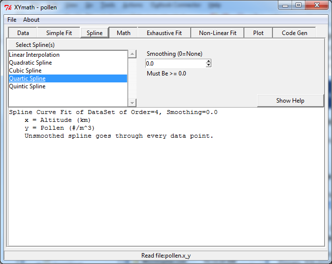
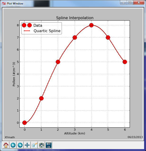
The graph below shows a spline that goes through every data point.
Math Operations
All math operations are limited to the X Range selected.
Select the equation of interest in the list box. Equations are generated in “Simple Fit”, “Spline”, “Exhaustive Fit” and “Non-Linear Fit”.
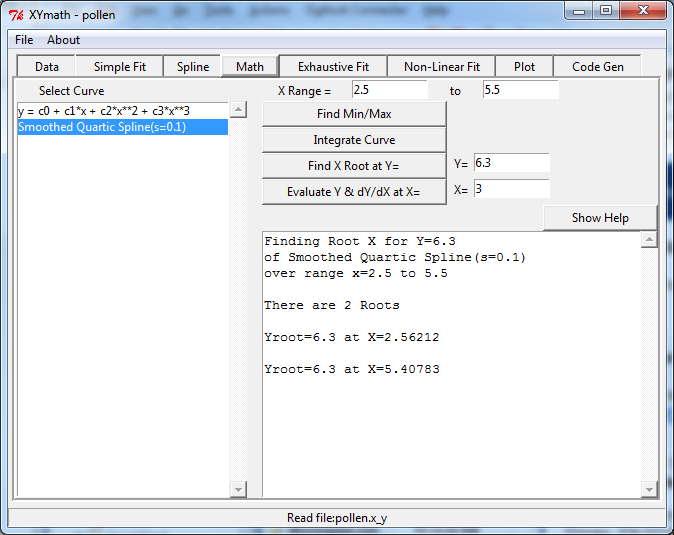
“Find Min/Max” will find the minimum and maximum y values in the X Range.
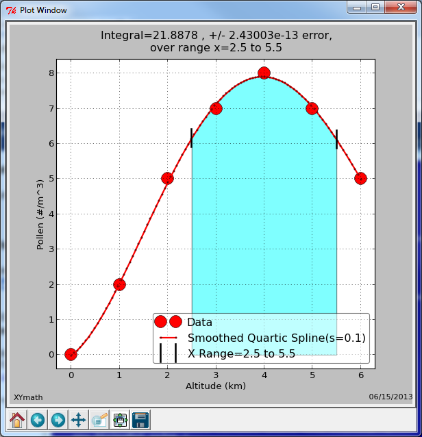
“Integrate Curve” will perform a numerical integration over the X Range.
“Find X Root at Y” will discover what value or values of x result in the desired value of y.
“Evaluate Y & dY/dX at X” will calculate the value of y as well as 1st and 2nd derivatives at the desired value of x.
An example of an integration plot is shown below.
Exhaustive Fit
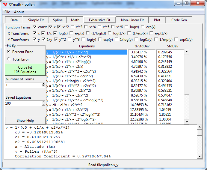
As for the Simple Fit, the X,Y data can be fit to equations by minimizing either total error, or percent error. Selecting the “Total Error” or “Percent Error” radio button will determine which approach is used.
Equations are generated by using all linear combinations of terms and transforms selected. Each equation has the number of terms selected.
Selecting function terms of “const”, “x” and “x**2” results in all combinations of those terms on the right hand side of the equations. Each of those x terms can be modified by x transforms.
Selecting x transforms of “x”, “1/x” and “log(x)” results in all terms using x being transformed into “x”, “1/x” or “log(x)”. For example “x**2” would become “x**2”, “1/x**2” or “log(x)**2”.
Selecting y transforms of “y”, “1/y” and “y**2” results in y=f(x), 1/y=f(x) and y**2=f(x) all being examined.
All of the equations are listed in order from best to worst standard deviation or percent standard deviation as appropriate.
By default, only the top 100 equations are listed, however, that can be changed with the “Saved Equations” selection box.
Note that for some equations, divide by zero is allowed if it results in (1/infinity) which is equal to 0.0
Non-Linear Fit
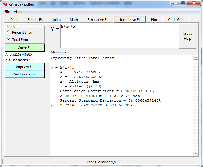
Any equation of the form y=f(x) may be entered and fit to the data here.
Enter ONLY the Right Hand Side of Your Equation (Assumed to be “y” equals a function of “x”. or “y=f(x)”)
For example to fit the equation “y = A*x**c” Enter: A*x**c
Notice that “x” must be lower case. Constants can be any mix of upper or lower case. Standard variable name rules apply. For example legal names include
A, c, mu, c8, theta, myConst, ZZZ, C3H8
Do NOT include “y” in the equation’s right hand side.
All constants start out with a value of 1.0 and are then optimized with a least squares approach to find the best values. Sometimes the optimization process will get stuck in a local optima. If this appears to be the case, edit the constant’s values and click “Set Constants”, followed by “Improve Fit”. If the equation form is a good one, this can result in a better curve fit.
Standard functions sin, cos, tan, log, log10, exp, sqrt, log1p, sinh, cosh and tanh are available.
Be aware that linear equations will also work correctly. for example enter “m*x + b” to fit a straight line.
As in “Simple Fit” and “Exhaustive Fit”, be sure to select either Percent or Total Error.
Note that for some equations, divide by zero is allowed if it results in (1/infinity) which is equal to 0.0
Plot
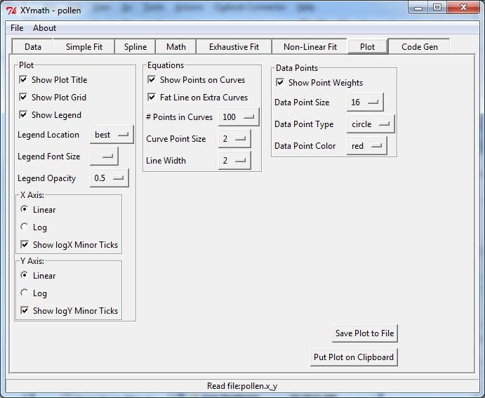
The plot can be modified in a number of ways as shown the Plot page below. In addition to modifying the plot, the plot can easily be saved to file or placed on the clipboard for pasting into an application such as PowerPoint or Word.
Code Generation
To Generate Code for the curve fit:
- Select the desired curve
- Select the desired language
- Press “Generate Code” button
This text box will be filled with the desired code which can then be copied and pasted into any text editor.
When copy to clipboard button appears, click it to place the source code on the computers clipboard for pasting into a text editor.
If Excel is selected, Excel will be launched and populated with the curve data.
All too often, the results of a curve fit are buried deep in an application’s source code without sufficient documentation to recreate, verify or update the equation. The source code generated by XYmath will answer those needs.
Another often neglected aspect of using curve fits is enforcing the fit’s range of applicability. The source code generated by XYmath will print warnings if the curve fit is called with an x value outside of the x data range.
Compiled FORTRAN can be imported into python through the use of the f2py utility that comes with numpy. The XYmath-generated FORTRAN code contains comments(“cf2py”) that help with the use of the f2py.
For example: python.exe -c “from numpy.f2py import main; main()” cfit.f -m cfit -h cfit.pyf will create an f2py definition file called “cfit.pyf” from a FORTRAN source file called “cfit.f”.
python.exe -c “from numpy.f2py import main; main()” cfit.pyf cfit.f will create a file called “cfit.pyd” that python can import with “import cfit”
See the f2py documentation for generating pyf and pyd files. Your machine may need special options such as “-c –compiler=mingw32” and/or “–fcompiler=gnu95” to define your FORTRAN compiler.

Below is an example of a FORTRAN routine generated by XYmath
C This FORTRAN Source Code Generated by XYmath

      SUBROUTINE curve_fit_sub( x, y )
      IMPLICIT DOUBLE PRECISION (A-H,O-Z)
      implicit integer (I-N)
      DOUBLE PRECISION x, y

C  set up f2py comments just in case a python import is desired
cf2py        DOUBLE PRECISION,INTENT(IN)::  x      ! Altitude (km)
cf2py        DOUBLE PRECISION,INTENT(OUT):: y      ! Pollen (#/m^3)

C  Curve Fit Results from XYmath 06/15/2013
C  y = A*x**c
C      A = 3.72169746285
C      c = 0.366745560992
C      x = Altitude (km)
C      y = Pollen (#/m^3)
C      Correlation Coefficient = 0.861093759115
C      Standard Deviation = 1.37150294436
C      Percent Standard Deviation = 36.6360457143%
C  y = 3.72169746285*x**0.366745560992

C (x,y) Data Pairs from 06/15/2013 Used in Curve Fit
C (x,y) = (0,0),(1,2),(2,5),(3,7),(4,8),(5,7),(6,5)


C  If input value of x is out of range, print warning
      IF (x.lt.0.0D0 .or. x.gt.6.0D0)THEN
        print*, 'WARNING... x is outside range in curve_fit_sub'
        print*, '  x =',x,' x range = (0.0D0 to 6.0D0)'
      ENDIF

      y = 3.72169746285D0*x**0.366745560992D0

      RETURN
      END
      PROGRAM TEST
      IMPLICIT DOUBLE PRECISION (A-H,O-Z)
      implicit integer (I-N)

      print*, '============================'
      call curve_fit_sub( 6.0D0, y_test )
      print*, 'y_test  =',y_test,'for x_test =',6.0D0
      print*, 'y_xymath=',7.1800022981D0
      print*, ' '
      print*, 'y_test should equal y_xymath above.'
      STOP
      END
